
Abstract
In recent years, reinforcement learning has witnessed substantial progress in domains such as robotics and Atari game-playing. Nevertheless, challenges related to data inefficiency and limited generalization capabilities have hindered further advancements in this field. Meta-reinforcement learning methods offer a promising solution by enabling policies to adapt to new tasks with fewer data samples compared to standard RL techniques. However, the meta-training phase itself demands a substantial amount of data and is costly. The incorporation of offline data into this process holds the potential to mitigate data inefficiency issues, yet it introduces its own set of complexities. In this review, we introduce various categories of offline meta-reinforcement learning approaches and provide an overview of relevant research papers within each category, facilitating a deeper understanding of this field.
Introduction
Meta-reinforcement learning refers to a group of machine learning techniques designed to acquire the ability to learn reinforcement learning itself. These methods have the potential to overcome the sample inefficiency of reinforcement learning methods during meta-test time. However, since these methods are trained on a distribution of similar tasks during meta-training, they require a greater amount of data, which implies that meta-training itself is sample inefficient but meta-testing is sample efficient [1].
Since meta-training requires a larger amount of data, online learning is not practical, and it could even be impossible in some cases since interaction with the environment may not be possible. Utilizing offline data in this situation could be a practical choice because the data is precollected and can alleviate the sample inefficiency problem.
However, offline reinforcement learning itself poses difficulties. The policy under which the offline data is collected ($\pi_b$) differs from the current learning policy ($\pi_{\theta}$), resulting in a discrepancy between the distributions of these two policies (distributional shift) [2]. This can be problematic when the agent selects an action that is not defined in $\pi_b$. In online learning, by interacting with the environment, the agent can rectify this difference; however, in offline settings, this difference cannot be overcome. Nonetheless, offline meta-reinforcement learning presents additional problems, the most important of which is that the distribution of trajectories seen by the agent during meta-testing and meta-training differs. However, within recent years, many approaches have been introduced to address this problem, which I introduce some of them in this literature review.
Preliminaries
In this section, we will introduce the mathematical formalism of reinforcement learning, alongside a brief introduction to meta-reinforcement learning and offline reinforcement learning.
Reinforcement Learning
A reinforcement learning algorithm learns a policy to interact in a Markov Decision Process, which is defined as a tuple $\mathcal{M} = (\mathcal{S}, \mathcal{A}, P, P_0, r, \gamma, T)$, where $\mathcal{S}$ is the state space, $\mathcal{A}$ is the action space, $P(s_{t+1}|s_t, a_t)$ is the transition probability from $s_t$ to $s_{t+1}$ after taking action $a_t$, $P_0$ is the initial state distribution, $r : \mathcal{S} \times \mathcal{A} \rightarrow \mathbb{R}$ is the reward function, $\gamma \in (0, 1]$ is a scalar discount factor, and $T$ is the horizon.
The policy $\pi(a | s) : \mathcal{M} \times \mathcal{A} \rightarrow \mathbb{R}_{+}$ is a distribution over actions conditioned on states. The interaction of the policy with the environment creates a distribution over trajectories, which is defined as:
\[\begin{equation} P(\tau) = P_0(s_0) \prod_{t=0}^{T} \pi(a_t|s_t) P(s_{t+1}|s_t, a_t) \end{equation}\]Using the trajectory distribution, the reinforcement learning objective (maximization of the expected discounted return), $J(\pi)$, can be written as:
\[\begin{equation} J{\pi} = \mathbb{E}_{\tau \sim P(\tau)} \sum_{t=0}^{T} \gamma^t r_t \end{equation}\]Meta-Reinforcement Learning
Meta-reinforcement learning utilizes a set of training tasks for acquiring a policy, which is capable of rapid adaptation to novel test tasks that were not encountered during the training phase. During the meta-training process, the learning algorithm is exposed to $M$ tasks, represented as ${\mathcal{T}_i}_1^M$, sampled from the task distribution $p(\mathcal{T})$. Subsequently, at meta-test time, a fresh task, denoted as $\mathcal{T}_j$ and drawn from $p(\mathcal{T})$, is randomly selected. This task was not previously encountered during meta-training, and the meta-trained policy must swiftly adapt to this new task in order to maximize its performance with a limited number of samples.
A proficient meta-reinforcement learning approach can meta-train a model that efficiently represents a highly effective reinforcement learning process. This trained model can subsequently tackle entirely novel tasks more quickly, significantly outperforming a traditional reinforcement learning algorithm that starts from scratch [3].
Offline Meta-Reinforcement Learning
Combining meta-reinforcement learning and offline reinforcement learning methods results in a new approach called offline meta-reinforcement learning, which can be categorized into two different groups of methods.
Optimization-Based Approaches
These approaches are based on MAML [4] and attempt to combine offline reinforcement learning methods with it. However, due to the properties of gradients required by MAML, this combination cannot be accomplished without additional modifications.
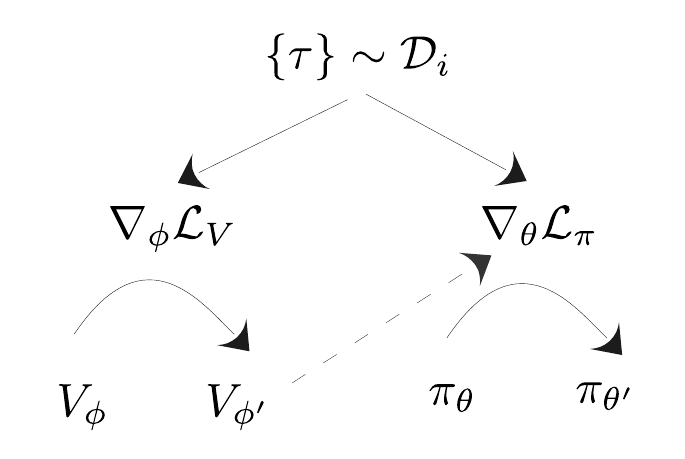
One of these approaches tries to combine Advantage Weighted Regression (AWR) [5], which consists of two supervised learning steps, with MAML. It uses Monte Carlo returns to learn a value function and a policy using the following loss functions:
\[\begin{equation} \mathcal{L}_V(\phi, \mathcal{D}_i) = \mathbb{E}_{s, a \sim \mathcal{D}_i} \begin{bmatrix} || \mathcal{R}_{s, a}^{\mathcal{D}} - V_{\phi}(s)||^2 \end{bmatrix} \end{equation}\] \[\begin{equation} \mathcal{L}_{AWR}(\theta, \phi, \mathcal{D}_i) = \mathbb{E}_{s, a \sim \mathcal{D}_i} \begin{bmatrix} -\log \pi_{\theta}(a|s) \exp \begin{pmatrix} \frac{1}{\beta} (\mathcal{R}_{\mathcal{D}_i} (s, a) - V_{\phi}(s)) \end{pmatrix} \end{bmatrix} \end{equation}\]Where \(\mathcal{D}_i=\{ s_{i, t}, a_{i, t}, s'_{i, t},r_{i, t} \}\) represents the collected trajectories from a policy, \(\mathcal{R}_{\mathcal{D}_i}(s, a)\) represents the Monte Carlo return for choosing action a in state s, $V_{\phi}(s)$ represents the learned value function, beta is a temperature value, and \(\mathcal{R}_{\mathcal{D}_i}(s, a) - V_{\phi}(s)\) represents the advantage.
In this approach, the value function is first updated using the Monte Carlo return, and subsequently, this learned value function is used in the policy update using $\mathcal{L}_{AWR}$.
 General AWR process.
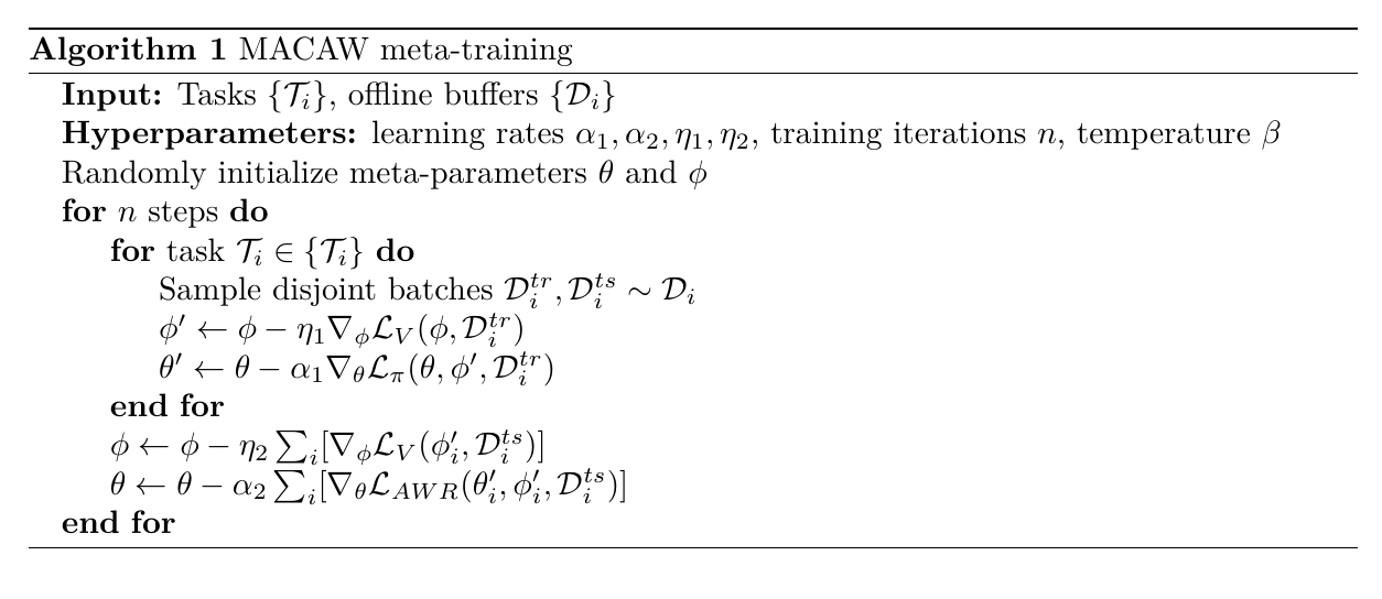
Meta-Actor Critic with Advantage Weighting (MACAW) [6] combines AWR with MAML to learn the values of $\theta$ and $\phi$ so that they can serve as initial parameters in meta-test, adapting to a new task with just a few gradient updates. Nevertheless, this approach necessitates additional modifications to function correctly. MAML requires universal loss functions [7], meaning that the inner gradient should contain all necessary information for task inference, but $\mathcal{L}_{AWR}$ is not universal. To tackle this problem, the MACAW policy update conducts both advantage-weighted regression onto actions and an additional regression onto advantages.
\[\begin{equation} \theta'_{i} \leftarrow \theta - \alpha_1 \nabla_{\theta} \mathcal{L}_{\pi}(\theta, \phi', \mathcal{D}_{i}^{tr}), \quad \text{where } \mathcal{L}_{\pi} = \mathcal{L}_{AWR} + \lambda \mathcal{L}_{ADV} \end{equation}\]which $\mathcal{L}_{ADV}$ is defined as:
\[\begin{equation} \mathcal{L}_{ADV}(\theta, \phi', \mathcal{D}) = \mathbb{E}_{s, a \sim \mathcal{D}} \begin{bmatrix} ||A_{\theta}(s, a) - (\mathcal{R}_{\mathcal{D}}(s, a) - V_{\phi'_{i}})||^2 \end{bmatrix} \end{equation}\]Finally, the meta-training phase can be formulated as shown in Algorithm 1.
Black-Box Approaches
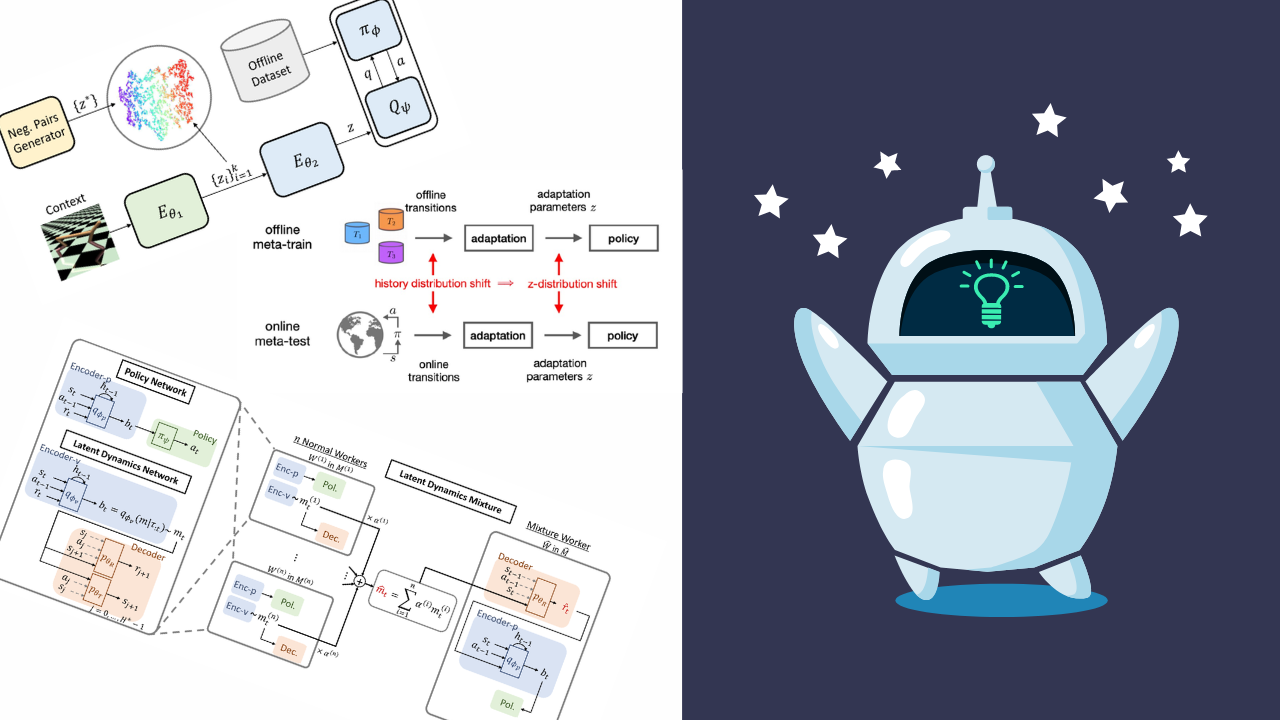
Also known as context-based approaches, these methods often use an encoder network to sample a context vector $\mathbf{z}$ from a distribution $q_{\phi_e}(\mathbf{z}|\mathcal{D})$. The policy $\pi_{\theta}(\mathbf{a}|\mathbf{s}, \mathbf{z})$ is then conditioned on both state $\mathbf{s}$ and context vector $\mathbf{z}$ by concatenating $\mathbf{z}$ to the state $\mathbf{s}$ [8]. However, these approaches face challenges with out-of-distribution (OOD) tasks. During meta-training, the offline data collected by an unknown policy is used for training, which means that the properties of offline trajectories are learned as context. However, during the meta-test, the agent interacts with the online environment and receives online trajectories, resulting in a distribution shift between meta-test and meta-train. Nonetheless, several methods have been introduced to mitigate this issue.
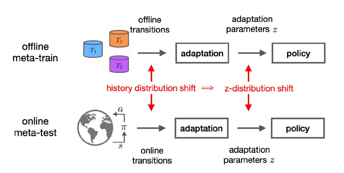 Image derived from [[8]](#8). out-of-distribution problem in context-based offline meta-learning approaches.
Using online trajectories in meta-training
Semi-supervised Meta Actor-Critic (SMAC) [8] uses offline data for meta-training alongside learning a reward function from existing offline labeled rewards. Then, the offline meta-reinforcement learning agent interacts with the environment to collect additional online data, but without labeled rewards. Instead, it uses the learned reward function from offline data to predict the online trajectory rewards to further meta-train using these data. The reward function is a decoder parametrized with $\phi_d$, designed for predicting the rewards, and its loss function is defined as:
\[\begin{equation} \mathcal{L}_{reward}(\phi_d, \phi_e, \tau, \mathbf{z}) = \sum_{(s, a, r) \in \tau} || r - r_{\phi_d}(s, a, \mathbf{z}) ||_{2}^{2} + D_{KL} \begin{pmatrix} q_{\phi_e}(\cdot|\tau) \hspace{1mm} \Big|\Big| \hspace{1mm}p_z(\cdot) \end{pmatrix} \end{equation}\]Latent Dynamics Mixture
Latent Dynamics Mixture (LDM) [9] combines offline trajectories to generate new trajectories, and comprises two separate networks. Similar to the previous approach, it includes an encoder $q_{\phi_p}$ that takes trajectories as input and produces a context on which the policy network is conditioned. The second network is the Latent Dynamics Network, which is composed of an encoder $q_{\phi_v}$ and two decoders $p_{\theta_R}$ and $p_{\theta_T}$. The encoder functions similarly to the encoder in the policy network, outputting the latent distribution $m_t \sim q_{\phi_v}(m|\tau_t)$ , while the decoders are conditioned on this latent information. During training, $n$ workers generate various latents $m_t^i \sim q_{\phi_v}(m|\tau_t^i)$ from different tasks. The weighted sum of these latents creates a new latent representation \(\hat{m}_t\). The reward decoder $p_{\theta_R}$ then utilizes this new latent representation to predict the corresponding reward $\hat{r}_t$. Finally, the policy leverages these new $\hat{m}_t$ and $\hat{r}_t$ values, which represent imaginary tasks, for further meta-training.
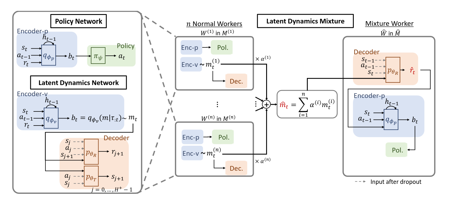 Image derived from [[9]](#9). General procedure of Latent Dynamics Mixture.
Better representations using Contrastive Learning
The goal of context-based approaches is to learn a representation for tasks. We observed that learning context is challenging in an offline setting, where the offline data is collected using an unknown policy. However, to improve the learning of task representations, some methods employ contrastive learning to enhance performance in out-of-distribution tasks.
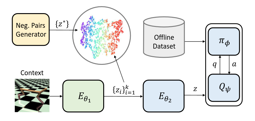 Image derived from [[10]](#10). CORRO general approach.
One of these methods is CORRO [10], which initially employs an encoder named the Transition Encoder, differing from previously encountered encoders. Instead of taking the entire trajectory as input, it processes one transition at a time and produces its context \(\mathbf{z}_i = E_{\phi_1}(s_{i, t}, a_{i, t}, s'_{i, t}, r_{i, t})\). Upon generating the context for all the transitions within a trajectory, another encoder known as the Aggregator combines them into a single context \(\mathbf{z} = E_{\phi_2}(\{ \mathbf{z}_i \}_{i=1}^{\tau})\). The transition encoder employs a contrastive loss to maximize mutual information for improved task representation, which its objective is defined as:
\[\begin{equation} \max_{\phi_1} \sum_{M_i \in \mathcal{M}-x, x'\in X_i} \begin{bmatrix} \log \begin{pmatrix} \cfrac{\exp(S(\mathbf{z}, \mathbf{z'}))}{\sum_{M^* \in \mathcal{M}} \exp(S(\mathbf{z}, \mathbf{z^*}))} \end{pmatrix} \end{bmatrix} \end{equation}\]Where $\mathcal{M}$ is the set of training tasks, $x$ and $x’$ (positive pairs) represent two transitions sampled from the same task distribution, and $\mathbf{z}$ and $\mathbf{z’}$ are the outputs of the transition encoder for these transitions. Moreover, \(x^*\) is sampled from a different set of data, indicating that $x$ and $x^*$ are negative pairs.
Another method that utilizes contrastive learning is DOMINO [11], which, instead of learning a single context, learns multiple decoupled contexts.
References
[1] J. Beck et al., “A survey of meta-reinforcement learning,” arXiv preprint arXiv:2301.08028, 2023.
[2] S. Levine, A. Kumar, G. Tucker, and J. Fu, “Offline reinforcement learning: Tutorial, review, and perspectives on open problems,” arXiv preprint arXiv:2005.01643, 2020.
[3] T. Yu et al., “Meta-world: A benchmark and evaluation for multi-task and meta reinforcement learning,” in Conference on robot learning, PMLR, 2020, pp. 1094–1100.
[4] C. Finn, P. Abbeel, and S. Levine, “Model-agnostic meta-learning for fast adaptation of deep networks,” in International conference on machine learning, PMLR, 2017, pp. 11261135.
[5] X. B. Peng, A. Kumar, G. Zhang, and S. Levine, “Advantage-weighted regression: Simple and scalable off-policy reinforcement learning,” arXiv preprint arXiv:1910.00177, 2019.
[6] E. Mitchell, R. Rafailov, X. B. Peng, S. Levine, and C. Finn, “Offline meta-reinforcement learning with advantage weighting,” in International Conference on Machine Learning, PMLR, 2021, pp. 7780–7791.
[7] C. Finn, “Learning to learn with gradients,” Ph.D. dissertation, EECS Department, University of California, Berkeley, Aug. 2018.
[8] V. H. Pong, A. V. Nair, L. M. Smith, C. Huang, and S. Levine, “Offline meta-reinforcement learning with online self-supervision,” in International Conference on Machine Learning, PMLR, 2022, pp. 17 811–17 829.
[9] S. Lee and S.-Y. Chung, “Improving generalization in meta-rl with imaginary tasks from latent dynamics mixture,” Advances in Neural Information Processing Systems, vol. 34, pp. 27 222–27 235, 2021.
[10] H. Yuan and Z. Lu, “Robust task representations for offline meta-reinforcement learning via contrastive learning,” in International Conference on Machine Learning, PMLR, 2022, pp. 25 747–25 759.
[11] Y. Mu et al., “Decomposed mutual information optimization for generalized context in meta-reinforcement learning,” arXiv preprint arXiv:2210.04209, 2022.
The pdf of the report is also available: