This post is also available on my colleague’s blog.
Abstract
In recent years, reinforcement learning has witnessed substantial progress in domains such as robotics and Atari game-playing. However, RL algorithms face challenges in terms of sample efficiency and exploration in complex and high-dimensional environments. Model-Based Reinforcement Learning represents a promising approach to address these challenges and enhance the efficiency and performance of RL algorithms.
Introduction
Usually, deep reinforcement learning algorithms demand a substantial number of training samples, leading to a considerably higher degree of sample complexity. In the context of RL tasks, sample inefficiency for a given algorithm quantifies the volume of samples needed to learn an approximately optimal policy. In contrast to supervised learning, which relies on historical labeled data for training, conventional RL algorithms rely on interaction data generated by executing the most up-to-date policy within the environment. Consequently, recent research in the realm of deep reinforcement learning has placed significant emphasis on enhancing sample efficiency [1].
In recent years, a series of papers known as Dreamers has been introduced, which are model-based RL agents that learn long-horizon behaviors from images solely through latent imagination. We begin by introducing the core concepts of DreamerV1, and we delve into DreamerV2 and DreamerV3, as well as other works based on Dreamer from other research groups, such as DreamerPro.
DreamerV1
The learning algorithm of DreamerV1 [2] is divided into two main parts: in the first one, the agent learns the latent dynamic model from the dataset of past experience to understand the environment’s dynamics, and in the second part, it learns the actor and critic models solely by envisioning the trajectories. In the end, the agent employs the learned action model to interact with the environment to gather more data for the first part.
Dynamics Learning
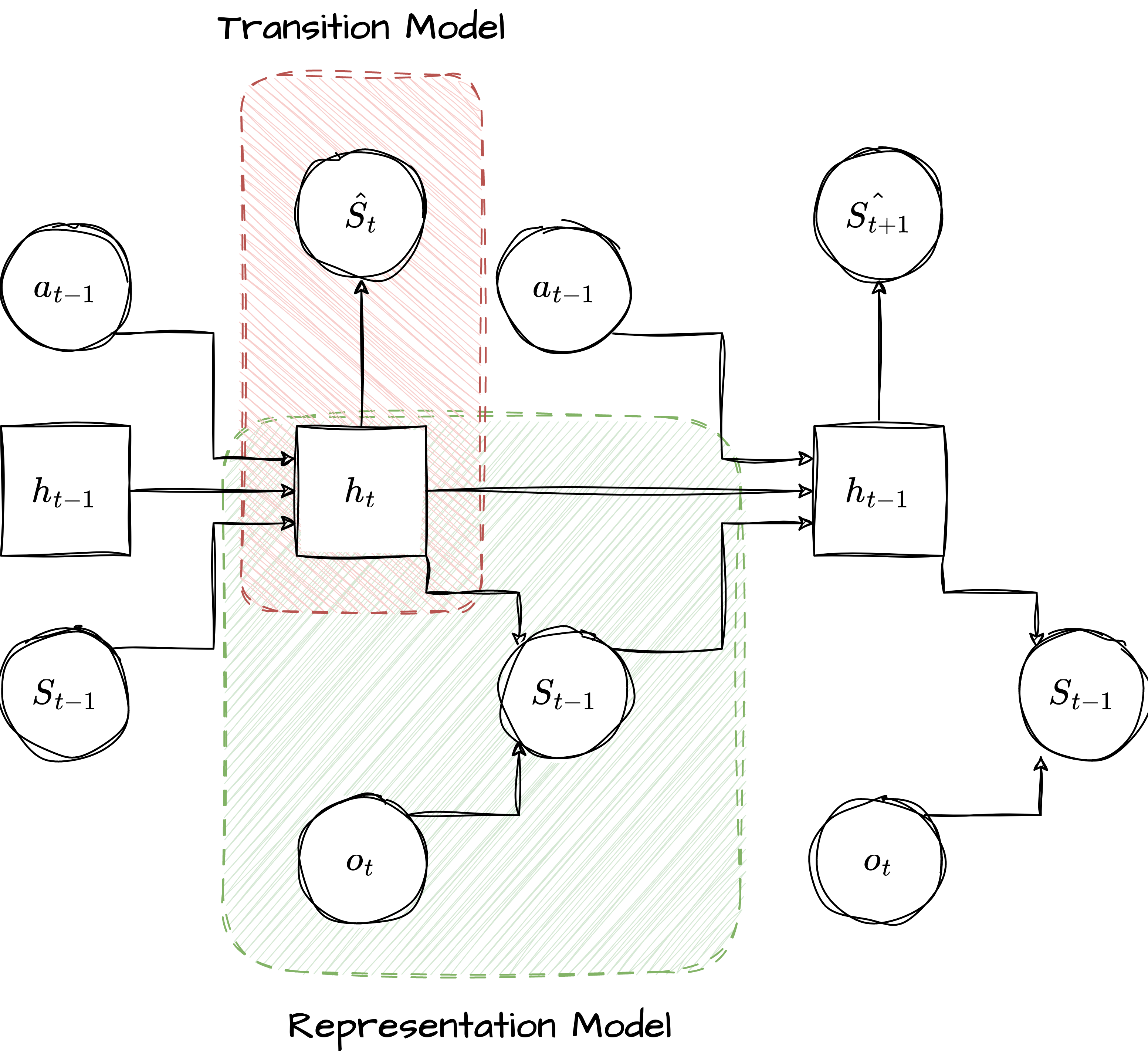
Dreamer learns a latent dynamics model comprising a representation model, a transition model, an observation model, and a reward model. Firstly, the representation model encodes the observation to generate state \(s_t\). Moreover, the transition model, which predicts ahead in the latent space, predicts future states solely by imagining the future, without interacting with the environment. The reward model predicts rewards based on the states, and the observation model attempts to reconstruct the input observation to enhance representation learning.
\[\begin{gather*} \begin{aligned} \begin{cases} \text{Representation Model:} & p_{\theta}(s_t | s_{t-1}, a_{t-1}, o_{t}) \\ \text{Observation Model:} & q_{\theta}(o_t | s_t) \\ \text{Reward Model:} & q_{\theta}(r_t | s_t) \\ \text{Transition Model:} & q_{\theta}(s_t | s_{t-1}, a_{t-1}) \end{cases} \end{aligned} \end{gather*}\] 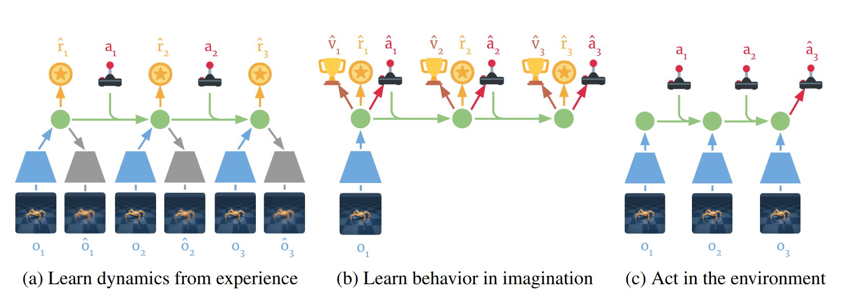 Dynamic learning in DreamerV1.
Initially, the dataset D is randomly initialized with random episodes. DreamerV1 learns latent dynamics by reconstructing input observations, which is beneficial when the dataset is finite or rewards are sparse. At each dynamics learning step, a batch of data is sampled from the dataset \(\mathcal{D}\), and the latent states are computed. Finally, to optimize the model’s parameters, the following loss function is utilized:
\[\begin{equation} \begin{aligned} & \mathcal{L}_{rec} = \mathcal{L}_{O}^{t} + \mathcal{L}_{R}^{t} + \mathcal{L}_{D}^{t} \\ & \mathcal{L}_{O}^{t} = \ln q(o_t | s_t) \\ & \mathcal{L}_{R}^{t} = \ln q(r_t | s_t) \\ & \mathcal{L}_{D}^{t} = -\beta KL \big(p(s_t | s_{t-1}, a_{t-1}, o_t) \big|\big| q(s_t|s_{t-1}, a_{t-1})\big) \end{aligned} \end{equation}\]Behavior Learning
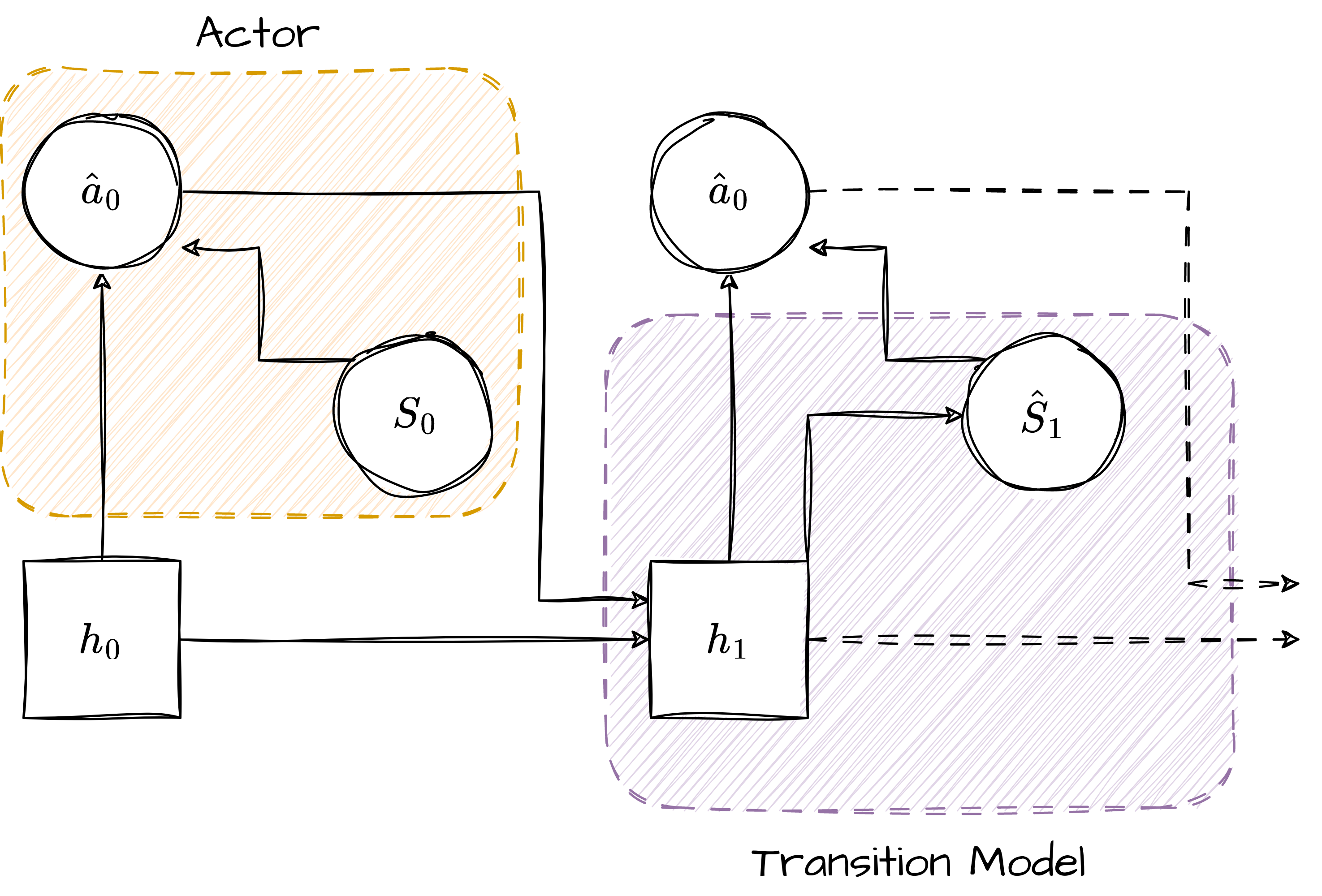
After the dynamic learning phase, the subsequent step involves learning the actor and critic using the acquired world model. The aim is to employ the model to “dream” the outcomes of actions without additional interactions with the environment. The process of simulation commences with a real observation, from which the latent state is derived using the representation model. This simulation continues for a finite horizon, and at each step, the agent selects an action based on the actor and computes the next latent state using the world model.
 Behavior learning in DreamerV1.
The process of behavior learning is depicted in Figure 2. As can be observed, the transition model is used in place of the representation model because the observations are not accessible during this phase.
DreamerV1 employs an actor-critic approach to learn behaviors. For that, it learns an action model and a value model within the latent space of the world model. The action model implements the policy and aims to predict actions that address the imagined environment, while the value model estimates the imagined return achieved from each state. The action and value models are trained cooperatively, following the typical policy iteration approach. The action model aims to maximize an estimate of the value, while the value model regresses towards the estimated value.
 Complete process of DreamerV1, image from [3].
DreamerV1 utilizes \(\lambda\)-return as its update target to balance bias and variance. As mentioned in [3], a valid update can be made not only towards any \(n\)-step return but also towards any average of \(n\)-step returns. \(\lambda\)-return is an exponentially weighted average of $n$-step returns, defined in DreamerV1 as follows:
\[\begin{equation} \begin{aligned} & V_{N}^{k}(s_{\tau}) \doteq \mathbb{E}_{q_{\theta}, q_{\phi}}\Big( \sum_{n=\tau}^{h-1} \gamma^{n-\tau} r_n + \gamma^{h-\tau} v_{\psi}(s_h) \Big), \quad \text{where} \quad h=\min(\tau+k, t+H),\\ & V_{\lambda}(s_\tau) \doteq (1-\lambda) \sum_{n=1}^{H-1} \lambda^{n-1} V_{N}^{n} (s_{\tau}) + \lambda^{H-1} V_{N}^{H}(s_{\tau }) \end{aligned} \end{equation}\] 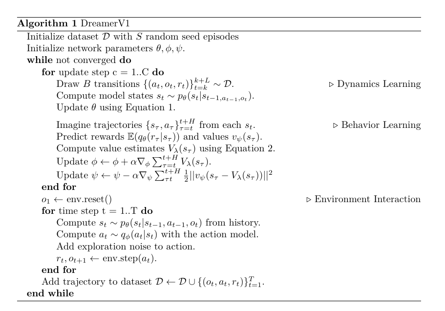
DreamerV2
DreamerV2 [4] builds upon the same model utilized in DreamerV1. During the training process, an encoder transforms each image into a representation that becomes integrated into the recurrent state of the world model. These representations lack access to perfect information about the images and instead focus on extracting only the essential elements needed for making predictions, thereby enhancing the agent’s resilience to unseen images. Subsequently, a decoder attempts to reconstruct the corresponding image, facilitating the acquisition of general representations. However, DreamerV2 applies new techniques to enhance the model’s learning, which we will introduce in this section.
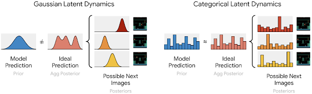 Image from official DreamerV2 blog, Gaussian and Categorical latent dynamics.
Categorical Variables
The first technique involves representing each image using categorical variables, as opposed to the Gaussian variables employed in DreamerV1. In this approach, the encoder transforms each image into 32 distributions, each consisting of 32 classes, the meanings of which are automatically determined as the world model learns. The one-hot vectors, drawn from these distributions, are then concatenated to create a sparse representation that is subsequently passed on to the recurrent state [4]. In contrast, earlier world models employing Gaussian predictors struggle to accurately capture the distribution over multiple Gaussian representations for the possible next images.
KL Balancing
DreamerV2 employs a loss function somewhat similar to DreamerV1. Nevertheless, it incorporates a technique known as KL balancing, which is applied to the KL loss term. The KL loss serves a dual role: it guides the prior towards the representations, while also imposing regularization on the representations in the direction of the prior. However, it is desired to prevent regularization towards an inadequately trained prior. DreamerV2 addresses this challenge by minimizing the KL loss more aggressively with respect to the prior compared to the representations, accomplished through the use of distinct learning rates.
Other changes have been implemented in DreamerV2, but the two mentioned above are the most significant. Nevertheless, for a comprehensive overview of these alterations, please refer to the appendix of the paper [4].
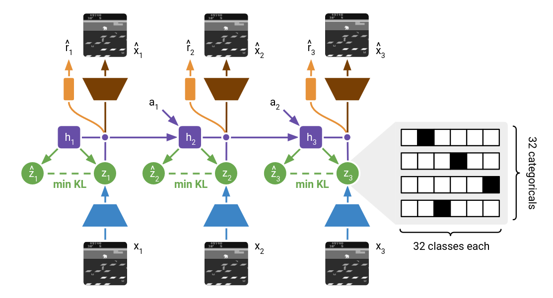 Image from [4], World model learning in DreamerV2.
DreamerV3
Similar to Dreamer1 and Dreamer2, Dreamer3 [5] also utilizes an RSSM to learn a model of the environment, which is further used by an actor-critic agent to learn a policy using imaginary trajectories. DreamerV3 is an improved version of DreamerV2 with several enhancements, the most important of which are described in the following subsections.
Symlog Predictions
To learn robustly across multiple domains, DreamerV3 learns a neural network that regresses onto the symlog (symmetric log) function defined as follows:
\[\text{symlog}_{x} = \text{sign}(x) \ln(|x| + 1)\] 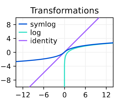 Image from [5], The symlog function compared to log and identity.
As can be seen in above, the symlog function compresses the magnitudes of both large positive and negative values, and unlike the logarithm, it is symmetric around the origin while preserving the input sign. DreamerV3 uses symlog predictions in the decoder, the reward predictor, and the critic, allowing this approach to robustly and quickly learn across a diverse range of environments.
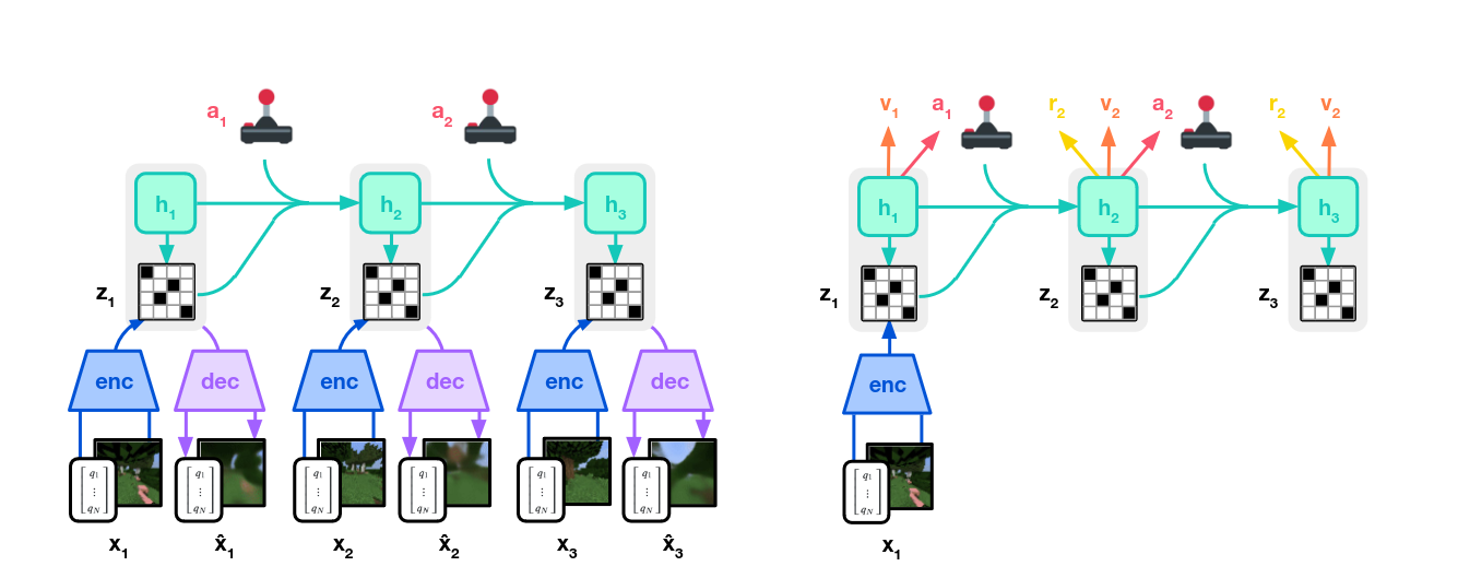 Image from [5], Training process of DreamerV3.
KL Regularizer
In DreamerV3, the world model parameters $\phi$ are optimized to minimize the following loss function:
\[\mathcal{L} = \beta_{pred} \mathcal{L}_{pred} + \beta_{dyn} \mathcal{L}_{dyn} + \beta_{rep} \mathcal{L}_{rep}\]where \(\beta_{pred} = 1\), \(\beta_{dyn} = 0.5\) and \(\beta_{rep} = 0.1\).
The prediction loss trains the decoder and reward predictor using the symlog loss. However, the dynamic and representation losses have been slightly modified from DreamerV2. A maximum term is added to the losses to prevent further learning when they are already minimized, directing the world model’s focus towards its prediction loss.
\[\mathcal{L}_{dyn} = \max (1, KL [sg(p(s_t | s_{t-1}, a_{t-1}, o_t)) || q(s_t|s_{t-1}, a_{t-1})])\] \[\mathcal{L}_{rep} = \max (1, KL [p(s_t | s_{t-1}, a_{t-1}, o_t) || sg(q(s_t|s_{t-1}, a_{t-1}))])\]Critic Learning
A simple choice for the critic loss function would be to regress the \(\lambda\)-returns via squared error or symlog predictions. However, the critic predicts the expected value of a potentially widespread return distribution, which can slow down learning. DreamerV3 utilizes a discrete regression approach for learning the critic based on twohot encoded targets. Twohot encoding is a generalization of one-hot encoding where all the bins are zero except the two closest to the input number. The sum of these bins should be zero, and more weight is given to the bin which is closest to the input number.
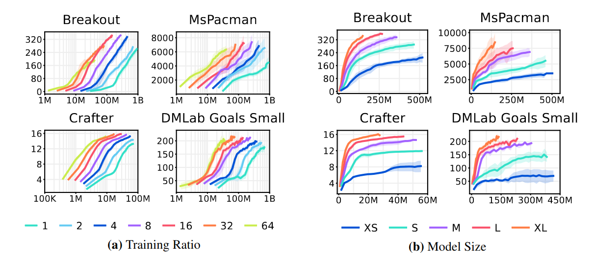 Image from [5], task performance over environment steps for different training ratios and model sizes. The training ratio is the ratio of replayed steps to environment steps. It can be seen that higher training ratios result in substantially improved data-efficiency, and larger models achieve not only higher final performance but also higher data-efficiency.
References
[1] F.-M. Luo, T. Xu, H. Lai, X.-H. Chen, W. Zhang, and Y. Yu, “A survey on model-based reinforcement learning,” arXiv preprint arXiv:2206.09328, 2022.
[2] D. Hafner, T. Lillicrap, J. Ba, and M. Norouzi, “Dream to control: Learning behaviors by latent imagination,” arXiv preprint arXiv:1912.01603, 2019.
[3] R. S. Sutton and A. G. Barto, Reinforcement learning: An introduction. MIT press, 2018.
[4] D. Hafner, T. Lillicrap, M. Norouzi, and J. Ba, “Mastering atari with discrete world models,” arXiv preprint arXiv:2010.02193, 2020.
[5] D. Hafner, J. Pasukonis, J. Ba, and T. Lillicrap, “Mastering diverse domains through world models,” arXiv preprint arXiv:2301.04104, 2023.
The pdf of the report is also available: